ISLR Chapter 8

ISLR Ch 8 #5, #7, #9

\(5\). Suppose we produce ten bootstrapped samples from a data set containing red and green classes. We then apply a classification tree to each bootstrapped sample and, for a specific value of X, produce 10 estimates of \(P (Class is Red|X)\):

0.1, 0.15, 0.2, 0.2, 0.55, 0.6, 0.6, 0.65, 0.7, and 0.75.

There are two common ways to combine these results together into a single class prediction. One is the majority vote approach discussed in this chapter. The second approach is to classify based on the average probability. In this example, what is the final classification under each of these two approaches?

The final classification under the Majority vote approach is that we classify \(X\) as red because 6 values had \(P > .5\) and 4 had values \(P < .5\) so the X is red. Using the average probability approach we classify \(X\) as green because the average of all the above probablilities is \(.45\) which is \(< .5\).

\(7.\) In the lab, we applied random forests to the Boston data using \(mtry = 6\) and using \(ntree = 25\) and \(ntree = 500\). Create a plot displaying the test error resulting from random forests on this data set for a more comprehensive range of values for mtry and ntree . You can model your plot after Figure 8.10. Describe the results obtained.

library(MASS)
library(randomForest)

set.seed(1)

n <- nrow(Boston)
train.set <- sample(1:n,n/2)

Boston.train <- Boston[train.set, -14]
Boston.test <- Boston[-train.set, -14]

Y.train <- Boston[train.set, 14]
Y.test <- Boston[-train.set, 14]

rf.a <- randomForest(Boston.train , Y.train, Boston.test, Y.test, mtry = ncol(Boston.train), ntree = 5000)
rf.b <- randomForest(Boston.train , Y.train, Boston.test, Y.test, mtry = ncol(Boston.train) / 2, ntree = 5000)
rf.c <- randomForest(Boston.train , Y.train, Boston.test, Y.test, mtry = sqrt(ncol(Boston.train)), ntree = 5000)

library(ggplot2)
ggplot() + 
  geom_line(aes(x = c(1:5000), y = rf.a$test$mse, color = "M = P")) +
  geom_line(aes(x = c(1:5000), y = rf.b$test$mse, color = "M = P/2")) +
  geom_line(aes(x = c(1:5000), y = rf.c$test$mse, color = "M = Sqrt(P)")) +
  theme_classic() + 
  xlab("Number of Trees") + ylab("Test Classification Error") + scale_colour_discrete(name="Form")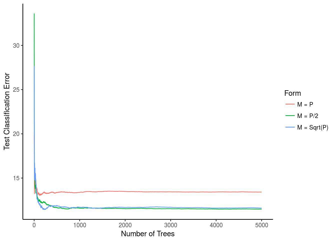

rf.a$test$mse[5000]

## [1] 13.41793

rf.b$test$mse[5000]

## [1] 11.49115

rf.c$test$mse[5000]

## [1] 11.60906

For M = P the classification error never got much better than \(~13.4%\), however for both \(M = P/2\) and \(M = \sqrt(P)\) the final error was much lower. both hovering right around 11.5% error. for \(M = \sqrt(P)\) the error actually reached that number when it had very few trees, but eventually it converged with the other model where \(M = P/2\)

\(9.\) This problem involves the OJ data set which is part of the ISLR package.

library(ISLR)

\((a)\) Create a training set containing a random sample of 800 observations, and a test set containing the remaining observations.

set.seed(2)
n <- nrow(OJ)
training.set <- sample(1:n, 800)
OJ.train <- OJ[training.set,]
OJ.test <- OJ[-training.set,]

\((b)\) Fit a tree to the training data, with \(Purchase\) as the response and the other variables as predictors. Use the summary() function to produce summary statistics about the tree, and describe the results obtained. What is the training error rate? How many terminal nodes does the tree have?

library(tree)
training.tree <- tree(Purchase ~ ., data = OJ.train)
summary(training.tree)

Classification tree: tree(formula = Purchase ~ ., data = OJ.train) Variables actually used in tree construction: [1] “LoyalCH” “PriceDiff” “ListPriceDiff” “PctDiscMM”
Number of terminal nodes: 8 Residual mean deviance: 0.7659 = 606.6 / 792 Misclassification error rate: 0.1675 = 134 / 800

The fitted tree has \(8 terminal nodes\) and has a \(training error rate of 0.1675\)

\((c)\) Type in the name of the tree object in order to get a detailed text output. Pick one of the terminal nodes, and interpret the information displayed.

training.tree

node), split, n, deviance, yval, (yprob) * denotes terminal node

1. root 800 1077.00 CH ( 0.60000 0.40000 )
   
2. LoyalCH < 0.50395 360 425.40 MM ( 0.27778 0.72222 )
   4. LoyalCH < 0.276142 176 132.60 MM ( 0.12500 0.87500 )
      
   5. LoyalCH < 0.0491775 63 10.27 MM ( 0.01587 0.98413 ) *
   6. LoyalCH > 0.0491775 113 108.50 MM ( 0.18584 0.81416 ) *
   7. LoyalCH > 0.276142 184 250.80 MM ( 0.42391 0.57609 )
      
   8. PriceDiff < 0.05 71 75.77 MM ( 0.22535 0.77465 ) *
   9. PriceDiff > 0.05 113 155.60 CH ( 0.54867 0.45133 ) *
3. LoyalCH > 0.50395 440 350.50 CH ( 0.86364 0.13636 )
   6. LoyalCH < 0.745156 182 210.00 CH ( 0.73626 0.26374 )
      
   7. ListPriceDiff < 0.235 70 97.04 CH ( 0.50000 0.50000 )
      24. PctDiscMM < 0.196196 51 66.22 CH ( 0.64706 0.35294 ) *
      25. PctDiscMM > 0.196196 19 12.79 MM ( 0.10526 0.89474 ) *
   8. ListPriceDiff > 0.235 112 80.42 CH ( 0.88393 0.11607 ) *
   9. LoyalCH > 0.745156 258 97.07 CH ( 0.95349 0.04651 ) *

The terminal node 13, is for \(ListPriceDiff > 0.235\) It has 102 observations and it has a deviance of \(80.42\). \(88.4%%\) of observations in this branch have a value of ‘CH’ and the remaining \(11.6%%\) take the value of MM

\((d)\) Create a plot of the tree, and interpret the results.

plot(training.tree)
text(training.tree)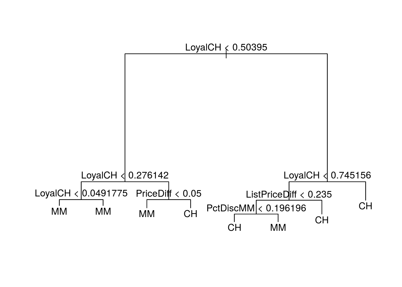

The root indicator of the tree is \(LoyalCH\), And it is again an important leaf node in several of the tree branches as an indicator variable for differentiating between CH and MM.

\((e)\) Predict the response on the test data, and produce a confusion matrix comparing the test labels to the predicted test labels. What is the test error rate?

library(magrittr)
test.pred <- predict(training.tree, OJ.test, type = "class")
prop.table(table(test.pred, OJ.test$Purchase)) %>% round(digits = 3)

##          
## test.pred    CH    MM
##        CH 0.596 0.104
##        MM 0.044 0.256

The test error rate is around \(23%%\)

\((f)\) Apply the cv.tree() function to the training set in order to determine the optimal tree size.

(cv.training.tree <- cv.tree(training.tree, FUN = prune.misclass))

## $size
## [1] 8 7 4 2 1
## 
## $dev
## [1] 150 148 172 172 320
## 
## $k
## [1]  -Inf   0.0   5.0   5.5 160.0
## 
## $method
## [1] "misclass"
## 
## attr(,"class")
## [1] "prune"         "tree.sequence"

\((g)\) Produce a plot with tree size on the x-axis and cross-validated classification error rate on the y-axis.

ggplot() + 
  geom_line(aes(x = cv.training.tree$size, y = cv.training.tree$dev)) + 
  geom_point(aes(x = cv.training.tree$size, y = cv.training.tree$dev), shape = 1, size = 2) +
  geom_text(aes(x = cv.training.tree$size, y = cv.training.tree$dev, label = cv.training.tree$dev), 
              nudge_y = 5, nudge_x = .25) +
  theme_classic() + 
  xlab("Tree Size") + ylab("CV Classification Error Rate")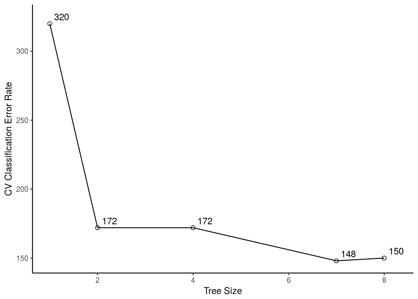

\((h)\) Which tree size corresponds to the lowest cross-validated classification error rate?

For this sample with \(set.seed(2)\) a tree with \(size = 7\) have the lowest CV Classification Error Rate.

\((i)\) Produce a pruned tree corresponding to the optimal tree size obtained using cross-validation. If cross-validation does not lead to selection of a pruned tree, then create a pruned tree with five terminal nodes.

pruned.tree <- prune.misclass(training.tree, best = 7)
plot(pruned.tree)
text(pruned.tree)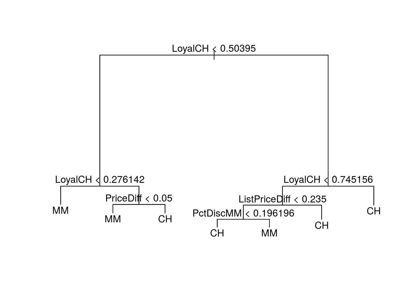

\((j)\) Compare the training error rates between the pruned and unpruned trees. Which is higher?

summary(training.tree)

Classification tree: tree(formula = Purchase ~ ., data = OJ.train) Variables actually used in tree construction: [1] “LoyalCH” “PriceDiff” “ListPriceDiff” “PctDiscMM”
Number of terminal nodes: 8 Residual mean deviance: 0.7659 = 606.6 / 792 Misclassification error rate: 0.1675 = 134 / 800

summary(pruned.tree)

Classification tree: snip.tree(tree = training.tree, nodes = 4L) Variables actually used in tree construction: [1] “LoyalCH” “PriceDiff” “ListPriceDiff” “PctDiscMM”
Number of terminal nodes: 7 Residual mean deviance: 0.7824 = 620.5 / 793 Misclassification error rate: 0.1675 = 134 / 800

Both Trees have an identical Misclassification error rate of \(0.1675\)

\((k)\) Compare the test error rates between the pruned and unpruned trees. Which is higher?

prune.pred <- predict(pruned.tree, OJ.test, type = "class")
prop.table(table(prune.pred,OJ.test$Purchase)) %>% round(digits = 3)

##           
## prune.pred    CH    MM
##         CH 0.596 0.104
##         MM 0.044 0.256

prop.table(table(test.pred, OJ.test$Purchase)) %>% round(digits = 3)

##          
## test.pred    CH    MM
##        CH 0.596 0.104
##        MM 0.044 0.256

Both have identical error rates and results. We removed one terminal node from the tree and the results were extremely simmilar. The Residual Mean Deviance Changed between the trees but besides that all else remained the same.