ISLR Ch3 Exercises #4, #15
- I collect a set of data (
n = 100 observations) containing a single predictor and a quantitative response. I then fit a linear regression model to the data, as well as a separate cubic regression, i.e. \(Y = \beta_{0}+\beta_{1}X+\beta_{2}X^{2}+\beta_{3}X^{3}+\epsilon\).
n = 100 observations) containing a single predictor and a quantitative response. I then fit a linear regression model to the data, as well as a separate cubic regression, i.e. \(Y = \beta_{0}+\beta_{1}X+\beta_{2}X^{2}+\beta_{3}X^{3}+\epsilon\).
\((a)\) Suppose that the true relationship between X and Y is linear, i.e. \(Y = \beta_0 + \beta_{1}X + \epsilon\). Consider the training residual sum of squares (RSS) for the linear regression, and also the training RSS for the cubic regression. Would we expect one to be lower than the other, would we expect them to be the same, or is there not enough information to tell? Justify your answer.
We would expect
RSSto be lower for thecubic regression. This model is much more flexible and will allow for the line to be much closer to the training data set.
\((b)\) Answer \((a)\) using test rather than training RSS.
We would expect the
RSSto be lower for thelinear regression. Since the true underlying relationship is linear the cubic regression is more likely to overpredict on the training set and therefor have a higherRSSfor the test set.
\((c)\) Suppose that the true relationship between X and Y is not linear, but we don’t know how far it is from linear. Consider the training RSS for the linear regression, and also the training RSS for the cubic regression. Would we expect one to be lower than the other, would we expect them to be the same, or is there not enough information to tell? Justify your answer.
The
cubic regressionmodel will perform better on the training set because it has greater degrees of freedom and the model is also non linear.
\((d)\) Answer \((c)\) using test rather than training RSS.
It is very possible that the
cubic regressionmodel will perform better on the test rather than the training data than thelinear regressionmodel but. If thecubic regressionmodel is over trained on the training data then thelinear regerssionmodel might strike a better line through the test data data and have a lowerRSS
- This problem involves the
Boston data set, which we saw in the lab for this chapter. We will now try to predict per capita crime rate using the other variables in this data set. In other words, per capita crime rate is the response, and the other variables are the predictors.
Boston data set, which we saw in the lab for this chapter. We will now try to predict per capita crime rate using the other variables in this data set. In other words, per capita crime rate is the response, and the other variables are the predictors.
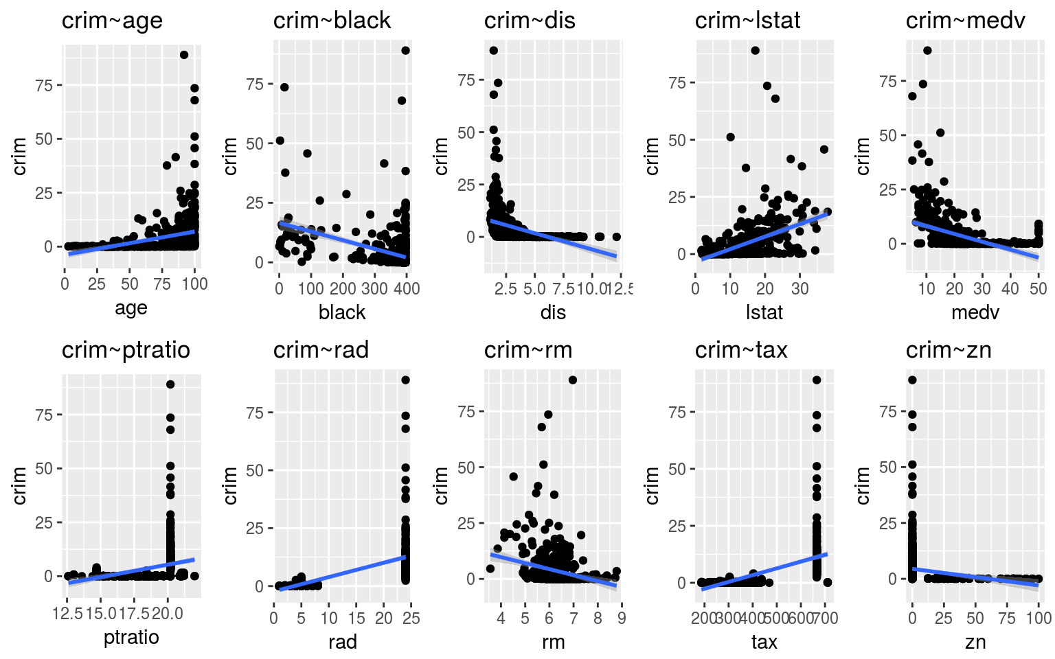
Boston <- MASS::Boston\((a)\) For each predictor, fit a simple linear regression model to predict the response. Describe your results. In which of the models is there a statistically significant association between the predictor and the response? Create some plots to back up your assertions.
library(magrittr)
lm.age     <- Boston %$% lm(crim~age)
lm.black   <- Boston %$% lm(crim~black)
lm.chas    <- Boston %$% lm(crim~chas)
lm.dis     <- Boston %$% lm(crim~dis)
lm.indus   <- Boston %$% lm(crim~indus)
lm.lstat   <- Boston %$% lm(crim~lstat)
lm.medv    <- Boston %$% lm(crim~medv)
lm.nox     <- Boston %$% lm(crim~nox)
lm.ptratio <- Boston %$% lm(crim~ptratio)
lm.rad     <- Boston %$% lm(crim~rad)
lm.rm      <- Boston %$% lm(crim~rm)
lm.tax     <- Boston %$% lm(crim~tax)
lm.zn      <- Boston %$% lm(crim~zn)
the following variables had a statistically signifigant associate between
crimand themselvesage,black,dis,lstat,medv,ptratio,rad,rm,tax,zn
\((b)\) Fit a multiple regression model to predict the response using all of the predictors. Describe your results. For which predictors can we reject the null hypothesis \(H_0\) : \(\beta_j = 0\)?
mult.reg.all <- lm(crim~., data=Boston)
pander(anova(mult.reg.all))| Df | Sum Sq | Mean Sq | F value | Pr(>F) | |
|---|---|---|---|---|---|
| zn | 1 | 1502 | 1502 | 36.21 | 3.457e-09 |
| indus | 1 | 4689 | 4689 | 113.1 | 6.469e-24 |
| chas | 1 | 247.8 | 247.8 | 5.976 | 0.01485 |
| nox | 1 | 1271 | 1271 | 30.65 | 5.041e-08 |
| rm | 1 | 138.5 | 138.5 | 3.341 | 0.0682 |
| age | 1 | 165.5 | 165.5 | 3.992 | 0.04628 |
| dis | 1 | 300.1 | 300.1 | 7.237 | 0.007383 |
| rad | 1 | 7238 | 7238 | 174.6 | 2.519e-34 |
| tax | 1 | 3.311 | 3.311 | 0.07984 | 0.7776 |
| ptratio | 1 | 7.281 | 7.281 | 0.1756 | 0.6754 |
| black | 1 | 455.3 | 455.3 | 10.98 | 0.000989 |
| lstat | 1 | 497.7 | 497.7 | 12 | 0.0005772 |
| medv | 1 | 447.9 | 447.9 | 10.8 | 0.001087 |
| Residuals | 492 | 20400 | 41.46 | NA | NA |
we can drop the following predictors,
tax,ptratio.rmis almost able to be rejected. Nextchasandageare on the chopping block. Lastlyageandmedvalso don’t have *** signifigance
\((c)\) How do your results from \((a)\) compare to your results from \((b)\)? Create a plot displaying the univariate regression coefficients from \((a)\) on the x-axis, and the multiple regression coefficients from \((b)\) on the y-axis. That is, each predictor is displayed as a single point in the plot. Its coefficient in a simple linear regression model is shown on the x-axis, and its coefficient estimate in the multiple linear regression model is shown on the y-axis.
from the plot you can see that
noxis varies quite a lot from theunivariate regression coefficients{\(31.25\)} to themultivariate regression coefficients{\(-10.32\)}
- Is there evidence of non-linear association between any of the predictors and the response? To answer this question, for each predictor X, fit a model of the form \(Y = \beta_{0} + \beta_{1}{X} + \beta_{2}{X}^{2} + \beta_{3}{X}^{3} + \epsilon\).
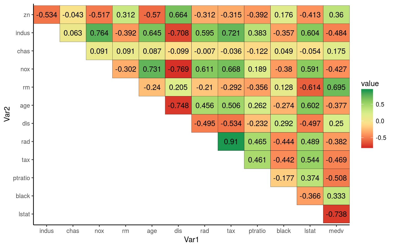
The colors represent how far apart two predictors are from eachother. For example when lstat is high medv is low. And when rad is high tax is also high. The more red something is the more they differ, and the more green something is the more they are simmilar. Yellow indicates that there is almost no correlation between the two variables.
\(age.\)
lm.age.d <- Boston %$% lm(crim~poly(age,3))
pander(summary(lm.age.d)$coefficients)| Estimate | Std. Error | t value | Pr(>|t|) | |
|---|---|---|---|---|
| (Intercept) | 3.614 | 0.3485 | 10.37 | 5.919e-23 |
| poly(age, 3)1 | 68.18 | 7.84 | 8.697 | 4.879e-17 |
| poly(age, 3)2 | 37.48 | 7.84 | 4.781 | 2.291e-06 |
| poly(age, 3)3 | 21.35 | 7.84 | 2.724 | 0.00668 |
the cubic polynomial is not statistically signifigant
\(black.\)
lm.black.d <- Boston %$% lm(crim~poly(black,3))
pander(summary(lm.black.d)$coefficients)| Estimate | Std. Error | t value | Pr(>|t|) | |
|---|---|---|---|---|
| (Intercept) | 3.614 | 0.3536 | 10.22 | 2.14e-22 |
| poly(black, 3)1 | -74.43 | 7.955 | -9.357 | 2.73e-19 |
| poly(black, 3)2 | 5.926 | 7.955 | 0.745 | 0.4566 |
| poly(black, 3)3 | -4.835 | 7.955 | -0.6078 | 0.5436 |
the cubic coefficient is not statistically signifigant
\(chas.\)
lm.chas.d <- Boston %$% lm(crim~poly(chas,1))
pander(summary(lm.chas.d)$coefficients)| Estimate | Std. Error | t value | Pr(>|t|) | |
|---|---|---|---|---|
| (Intercept) | 3.614 | 0.3822 | 9.455 | 1.216e-19 |
| poly(chas, 1) | -10.8 | 8.597 | -1.257 | 0.2094 |
can only be evaulated to one degree because
chasis a boolean variable (1’s and 0’s) and it is not statistically signifigant
\(dis.\)
lm.dis.d <- Boston %$% lm(crim~poly(dis,3))
pander(summary(lm.dis.d)$coefficients)| Estimate | Std. Error | t value | Pr(>|t|) | |
|---|---|---|---|---|
| (Intercept) | 3.614 | 0.3259 | 11.09 | 1.06e-25 |
| poly(dis, 3)1 | -73.39 | 7.331 | -10.01 | 1.253e-21 |
| poly(dis, 3)2 | 56.37 | 7.331 | 7.689 | 7.87e-14 |
| poly(dis, 3)3 | -42.62 | 7.331 | -5.814 | 1.089e-08 |
all three polynomials are statistically signifigant
\(indus.\)
lm.indus.d <- Boston %$% lm(crim~poly(indus,3))
pander(summary(lm.indus.d)$coefficients)| Estimate | Std. Error | t value | Pr(>|t|) | |
|---|---|---|---|---|
| (Intercept) | 3.614 | 0.33 | 10.95 | 3.606e-25 |
| poly(indus, 3)1 | 78.59 | 7.423 | 10.59 | 8.854e-24 |
| poly(indus, 3)2 | -24.39 | 7.423 | -3.286 | 0.001086 |
| poly(indus, 3)3 | -54.13 | 7.423 | -7.292 | 1.196e-12 |
the square polynomial is not statistically signifigant
\(lstat.\)
lm.lstat.d <- Boston %$% lm(crim~poly(lstat,3))
pander(summary(lm.lstat.d)$coefficients)| Estimate | Std. Error | t value | Pr(>|t|) | |
|---|---|---|---|---|
| (Intercept) | 3.614 | 0.3392 | 10.65 | 4.939e-24 |
| poly(lstat, 3)1 | 88.07 | 7.629 | 11.54 | 1.678e-27 |
| poly(lstat, 3)2 | 15.89 | 7.629 | 2.082 | 0.0378 |
| poly(lstat, 3)3 | -11.57 | 7.629 | -1.517 | 0.1299 |
the square and cubic polynomials are not statistically signifigant
\(medv.\)
lm.medv.d <- Boston %$% lm(crim~poly(medv,3))
pander(summary(lm.medv.d)$coefficients)| Estimate | Std. Error | t value | Pr(>|t|) | |
|---|---|---|---|---|
| (Intercept) | 3.614 | 0.292 | 12.37 | 7.024e-31 |
| poly(medv, 3)1 | -75.06 | 6.569 | -11.43 | 4.931e-27 |
| poly(medv, 3)2 | 88.09 | 6.569 | 13.41 | 2.929e-35 |
| poly(medv, 3)3 | -48.03 | 6.569 | -7.312 | 1.047e-12 |
all three polynomials are statistically signifigant
\(nox.\)
lm.nox.d <- Boston %$% lm(crim~poly(nox,3))
pander(summary(lm.nox.d)$coefficients)| Estimate | Std. Error | t value | Pr(>|t|) | |
|---|---|---|---|---|
| (Intercept) | 3.614 | 0.3216 | 11.24 | 2.743e-26 |
| poly(nox, 3)1 | 81.37 | 7.234 | 11.25 | 2.457e-26 |
| poly(nox, 3)2 | -28.83 | 7.234 | -3.985 | 7.737e-05 |
| poly(nox, 3)3 | -60.36 | 7.234 | -8.345 | 6.961e-16 |
all three polynomials are statistically signifigant
\(ptratio.\)
lm.ptratio.d <- Boston %$% lm(crim~poly(ptratio,3))
pander(summary(lm.ptratio.d)$coefficients)| Estimate | Std. Error | t value | Pr(>|t|) | |
|---|---|---|---|---|
| (Intercept) | 3.614 | 0.361 | 10.01 | 1.271e-21 |
| poly(ptratio, 3)1 | 56.05 | 8.122 | 6.901 | 1.565e-11 |
| poly(ptratio, 3)2 | 24.77 | 8.122 | 3.05 | 0.002405 |
| poly(ptratio, 3)3 | -22.28 | 8.122 | -2.743 | 0.006301 |
the cubic polynomial is not statistically signifigant, and the square polynomial is barely statistically signifigant
\(rad.\)
lm.rad.d <- Boston %$% lm(crim~poly(rad,3))
pander(summary(lm.rad.d)$coefficients)| Estimate | Std. Error | t value | Pr(>|t|) | |
|---|---|---|---|---|
| (Intercept) | 3.614 | 0.2971 | 12.16 | 5.15e-30 |
| poly(rad, 3)1 | 120.9 | 6.682 | 18.09 | 1.053e-56 |
| poly(rad, 3)2 | 17.49 | 6.682 | 2.618 | 0.009121 |
| poly(rad, 3)3 | 4.698 | 6.682 | 0.7031 | 0.4823 |
the cubic polynomial is not statistically signifigant, and the square polynomial is barely statistically signifigant, less so than for ptratio
\(rm.\)
lm.rm.d <- Boston %$% lm(crim~poly(rm,3))
pander(summary(lm.rm.d)$coefficients)| Estimate | Std. Error | t value | Pr(>|t|) | |
|---|---|---|---|---|
| (Intercept) | 3.614 | 0.3703 | 9.758 | 1.027e-20 |
| poly(rm, 3)1 | -42.38 | 8.33 | -5.088 | 5.128e-07 |
| poly(rm, 3)2 | 26.58 | 8.33 | 3.191 | 0.001509 |
| poly(rm, 3)3 | -5.51 | 8.33 | -0.6615 | 0.5086 |
the cubic polynomial is not statistically signifigant, and the square polynomial is just almost statistically signifigant but not quite
\(tax.\)
lm.tax.d <- Boston %$% lm(crim~poly(tax,3))
pander(summary(lm.tax.d)$coefficients)| Estimate | Std. Error | t value | Pr(>|t|) | |
|---|---|---|---|---|
| (Intercept) | 3.614 | 0.3047 | 11.86 | 8.956e-29 |
| poly(tax, 3)1 | 112.6 | 6.854 | 16.44 | 6.976e-49 |
| poly(tax, 3)2 | 32.09 | 6.854 | 4.682 | 3.665e-06 |
| poly(tax, 3)3 | -7.997 | 6.854 | -1.167 | 0.2439 |
the cubic polynomial is not statistically signifigant
\(zn.\)
lm.zn.d <- Boston %$% lm(crim~poly(zn,3))
pander(summary(lm.zn.d)$coefficients)| Estimate | Std. Error | t value | Pr(>|t|) | |
|---|---|---|---|---|
| (Intercept) | 3.614 | 0.3722 | 9.709 | 1.547e-20 |
| poly(zn, 3)1 | -38.75 | 8.372 | -4.628 | 4.698e-06 |
| poly(zn, 3)2 | 23.94 | 8.372 | 2.859 | 0.004421 |
| poly(zn, 3)3 | -10.07 | 8.372 | -1.203 | 0.2295 |
the cubic polynomial is not statistically signifigant, and the square polynomial is almost statistically signifigant
There is a possibility of a non linear relationship for
indus,medvand,noxwithcrim. `